Project Report
Motivation
As NBA fans, we are witnessing probably the greatest revolution ever on the court, which is called “Small ball era”. Teams tend to use small and faster players instead of traditional giants to accelerate moving speed and improve shooting efficiency.
Last year, Knicks, the home team of New York, returned to playoff season after eight years(link), which brought great joy to the fans. In order to make this performance long-lasting, we feel obligated to research the key variables that contribute to the winning so that help Knicks maintain existing strengths and make up for the shortages.
The most obvious feature of the current “small ball era” is the lifting of speed and the rise of 3 point shot attempt. In this way, we focus on three-point related variables along with other factors to conduct our analysis.
Questions
To get into playoff season, a team need to rank top eight among the fifteen teams in either east or west conference. The rank of team is determined by the number of games that a team win in a regular season. Therefore, we are going to explore how the number of games won by a team is associated with parameters evaluating average performance and give suggestions on the improvement of these abilities.
What is the threshold number of wins to enter playoff?
At the very beginning, we are interested in exploring the distribution of the number of games won by NBA playoff teams to find the threshold number of wins to enter into the playoff.Which variables contribute to the total wins of a season and a single game winning?
Then We want to figure out the factors contributing to total wins of a season and single win of a game. With the assumption that total wins are independent between each team and each year, and the result of a single game is independent of another, we conducted two regressions. One used linear regression model to fit total wins with average performance predictors. The other used stats per game to predict the win or lose of a single game.Will Knicks get into play-off according to the current model prediction?
In addition, we would use our model and the new data to predict the number of wins of Knicks in this 2021-22 season, and to see whether it can get into play-off season.What is the difference in average performance between Knicks and top teams?
Then according to the regression results, we want to analyse the performance of Knicks on key predictors to see the advantages and shortages of Knicks.which specific players cause these shortages and how to improve the overall performance?
Finally, we deep dived these gaps from team level into player level and found how leading players should improve to get more wins. A detailed game and training strategy is proposed.
Data
Data Source
As our project needs detailed stats about NBA teams and players from last 10 seasons NBA regular season, we used scrapping to get official advanced data from NBA Stats. There are four datasets we mainly used:
Advanced Box Score: In this data set, each observation represent a game and the specific data in this game, which contains the score, total field goal attempt, three point made and so on.
Playtype by Team: this data set contains average data for each team of a season in the aspect of offensive play type, such as isolation, pick and roll, ect. Each observation represent the team average data in a regular season with respect to a specific play type.
Tracking: this data set contains detailed information about NBA teams’ average movement data in a regular season, for example, passing, touches.
Knicks Shooting Log: in this data set, each observation represent a field goal that player in Knicks made, including the player who made the shot, the location they shot, the time remaining when the shot was made.
As I mentioned above, these data sets were scrapped from NBA website, the code to scrap data can be found at scrapping data
Data Wrangling
Data scrapping
We met with a huge problem at the very beginning that the most detailed NBA Stats website do not have API for scrapping. So we learned from Phillips’ blog to write a function to extract data using web devtools.The code we wrote can be found here. In the meantime, the last column of every dataset on that website is NA, so we exclude it.
scrapping_data = function(url) {
  headers = headers = c(
  `Connection` = 'keep-alive',
  `Accept` = 'application/json, text/plain, */*',
  `x-nba-stats-token` = 'true',
  `X-NewRelic-ID` = 'VQECWF5UChAHUlNTBwgBVw==',
  `User-Agent` = 'Mozilla/5.0 (Macintosh; Intel Mac OS X 10_15_7) AppleWebKit/537.36 (KHTML, like Gecko) Chrome/95.0.4638.69 Safari/537.36',
  `x-nba-stats-origin` = 'stats',
  `Sec-Fetch-Site` = 'same-origin',
  `Sec-Fetch-Mode` = 'cors',
  `Referer` = 'https://stats.nba.com/players/leaguedashplayerbiostats/',
  `Accept-Encoding` = 'gzip, deflate, br',
  `Accept-Language` = 'en-US,en;q=0.9')
  response = GET(url, add_headers(headers))
  data = fromJSON(content(response, as = "text"))
  df = data.frame(data$resultSets$rowSet[[1]], stringAsFactors = FALSE)
  names(df) = tolower(data$resultSets$headers[[1]])
  return(df)
}

drop_last_column = function(df) {
  df = df %>% select(-names(df)[[length(names(df))]])
  return(df)}
Next, because the knitting time is too long due to scrapping process, we extracted the datasets and variables we want and saved them to local for further use. There were seven datasets extracted in total. Here is one example datasets, box_score_all.
season_years = c("2020-21", "2019-20",
           "2018-19", "2017-18",
           "2016-17", "2015-16",
           "2014-15", "2013-14",
           "2012-13", "2011-12",
           "2010-11", "2009-10",
           "2008-09", "2007-08",
           "2006-07", "2005-06",
           "2004-05", "2003-04",
           "2002-03", "2001-02")

box_score_all = tibble(
  season_year = season_years,
  url = str_c("https://stats.nba.com/stats/teamgamelogs?DateFrom=&DateTo=&GameSegment=&LastNGames=0&LeagueID=00&Location=&MeasureType=Base&Month=0&OpponentTeamID=0&Outcome=&PORound=0&PaceAdjust=N&PerMode=Totals&Period=0&PlusMinus=N&Rank=N&Season=", season_year, "&SeasonSegment=&SeasonType=Regular+Season&ShotClockRange=&VsConference=&VsDivision="),
  box_score = map(url, scrapping_data)) %>%
  mutate(box_score = map(box_score, drop_last_column)) %>% # last column of each box score is NA
  select(-season_year, -url) %>%
  unnest(cols = box_score)

write_csv(box_score_all, "./data2/box_score_all.csv")
In this way, we just need to read them and select related variables every time we used them.
box_score_all = read_csv("./data2/box_score_all.csv") %>%
  janitor::clean_names() %>%
  select(-contains("rank"))

pass_df =
  read_csv("./data2/pass_df.csv") %>%
  select(season_year, team_abbreviation, passes_made)

isol_df =
  read_csv("./data2/isol_df.csv") %>%
  select(season_year, team_abbreviation, poss) %>%
  rename(poss_iso = poss)

prbh_df =
  read_csv("./data2/prbh_df.csv") %>%
  select(season_year, team_abbreviation, poss) %>%
  rename(poss_prb = poss)

prrm_df =
  read_csv("./data2/prrm_df.csv") %>%
  select(season_year, team_abbreviation, poss) %>%
  rename(poss_prr = poss)

defend_df =
  read_csv("./data2/defensive_impact_df.csv") %>%
  select(season_year, team_abbreviation, stl, blk, dreb)

trans_df =
  read_csv("./data2/transition_df.csv") %>%
  select(season_year, team_abbreviation, poss) %>%
  rename(poss_trans = poss)
As these are raw datasets documented by game, we need to do some summarizing, variable adding and deletion for different use.
Average Data Frame
The avg_df contains the number of wins by team and year in the last 20 years, which is used to analyse the distribution of threshold wins, and to further generate predict_df for regression.
Wrangling process:
Firstly, select the variables we are interested from box_score_all.
Secondly, define four new variables.
* win: changed w/l in wl into 1/0, making it easier to calculate the total number of wins. 1 means winning and 0 means lost.
* game_num: constant 1, which is used to calculate the number of games played.
* fg3a_p: the percentage of 3 point field goal attempt in total shooting attempt.
* conference: change historical team name to current abbreviation and define west or east according to team abbreviation.
Thirdly, do some summarizing. * calculate total number of wins, total number of games, total number of field goal attempt, total number of field goal made, total number of 3 points field goal attempt and total number of 3 points field goal made by team and season.
* calculate average number of points, average number of assists and average number of turnovers by team and season.
* standardlize the number of wins in strike season and COVID-19 season.
* arrange all data by season year and number of wins.
* rank calculate the rank in east or west conference by team and year
* play_off_team marked whether or not a team entered into the playoff in that year
* relocate key variables at the first.
avg_df =
  box_score_all %>%
  select(season_year, team_abbreviation, wl, pts, ast, tov, fgm, fga, fg3m, fg3a) %>%
  mutate(
    win = case_when(wl == "W" ~ 1, TRUE~0),
    game_num = 1,
    team_abbreviation = str_replace(team_abbreviation, "NOH", "NOP"),
    team_abbreviation = str_replace(team_abbreviation, "NJN", "BKN"),
    conference = case_when(
      team_abbreviation %in% c("UTA","PHX","LAC","DEN","DAL","LAL","POR","GSW","SAS","MEM","NOP","SAC","MIN","OKC","HOU","SEA","NOK","CHH")~"west",
      team_abbreviation %in% c("PHI","BKN","MIL","ATL","NYK","MIA","BOS","IND","WAS","CHI","TOR","CLE","ORL","DET","CHA")~"east") # divide into east and west conference
    ) %>%
  group_by(season_year, team_abbreviation, conference) %>%
  summarise(
    wins = sum(win),
    games = sum(game_num),
    games_should = 82,
    pts_avg = round(mean(pts), digits = 1),
    ast_avg = round(mean(ast), digits = 1),
    tov_avg = round(mean(tov), digits = 1),
    fgm_total = sum(fgm),
    fga_total = sum(fga),
    fg3m_total = sum(fg3m),
    fg3a_total = sum(fg3a)
    ) %>%
  mutate(
    wins_revised = round(wins/games*games_should,0),# due to labor negotiation in 2011-12, COVID-19.
    fg3_p = fg3a_total/fga_total,
    fg3_r = fg3m_total/fg3a_total
    ) %>%
  arrange(desc(season_year),desc(wins)) %>%
  group_by(season_year,conference) %>%
  mutate(
    conf_rank = row_number(),
    play_off_team = case_when(
           conf_rank <= 8 ~ "playoff",
           conf_rank > 8 ~ "non-playoff"
         ),
         play_off_team = fct_relevel(play_off_team, c("playoff", "non-playoff"))) %>%
  relocate(season_year, team_abbreviation, conference, wins, wins_revised, everything())
Predict Data Frame
The predict_df contain the average performance data with total number of games won in the last 8 years, which is used to build models and predict the number of winnings.
Wrangling process:
Firstly, combine the avg_df with 6 other dataframes to include playtype data and defensive data together with fundamental average stats like points, steals, blocks and turnovers from avg_df.
Secondly, drop the data before 2012-2013 season, which is not included in some datasets.
Thirdly, delete variables not related with regression.
predict_df =
  avg_df %>%
  left_join(defend_df, by = c("season_year","team_abbreviation")) %>%
  left_join(prrm_df, by = c("season_year","team_abbreviation")) %>%
  left_join(prbh_df, by = c("season_year","team_abbreviation")) %>%
  left_join(isol_df, by = c("season_year","team_abbreviation")) %>%
  left_join(pass_df, by = c("season_year","team_abbreviation")) %>%
  left_join(trans_df, by = c("season_year","team_abbreviation")) %>%
  drop_na(poss_trans, passes_made, poss_iso, poss_prb, poss_prr, stl, blk, dreb) %>%
  mutate(
    poss_pr = poss_prr + poss_prb
  ) %>%
  select(-poss_prr, -poss_prb, -wins, -games, -games_should, -fgm_total, -fga_total)
Box Score Data Frame for Visualization
This dataframe contains 23476 observations in the last 8 years which is mainly used for analyzing the tendency of different stats between playoff teams and non-playoff teams.
Wrangling process:
Firstly, apply the wrangling process from avg_df in game level.
Secondly, get conf_rank dataframe and join the box_score_viz with rank data.
box_score_viz =
  box_score_all %>%
  filter(season_year %in% c("2011-12", "2012-13", "2013-14", "2014-15", "2015-16", "2016-17", "2017-18", "2018-19", "2019-20", "2020-21")) %>%
  mutate(team_abbreviation = str_replace(team_abbreviation, "NOH", "NOP"),
    team_abbreviation = str_replace(team_abbreviation, "NJN", "BKN")) %>%
  select(season_year, team_abbreviation, wl, pts, ast, tov, fgm, fga, fg3m, fg3a, stl, blk, dreb) %>%
  mutate(
    win = case_when(wl == "W" ~ 1, TRUE~0),
    game_num = 1,
    conference = case_when(
      team_abbreviation %in% c("UTA","PHX","LAC","DEN","DAL","LAL","POR","GSW","SAS","MEM","NOP","SAC","MIN","OKC","HOU","SEA","NOK","CHH")~"west",
      team_abbreviation %in% c("PHI","BKN","MIL","ATL","NYK","MIA","BOS","IND","WAS","CHI","TOR","CLE","ORL","DET","CHA")~"east"), # divide into east and west conference
    fg3a_p = round(fg3a/fga, digits = 3),
    fg3_r = round(fg3m/fg3a, digits = 3)
    ) %>%
  relocate(season_year, team_abbreviation, conference)

conf_rank =
  avg_df %>%
  filter(season_year %in% c("2011-12", "2012-13", "2013-14", "2014-15", "2015-16", "2016-17", "2017-18", "2018-19", "2019-20", "2020-21")) %>%
  ungroup() %>%
  select(season_year, team_abbreviation, conference, conf_rank)


#join the two table together
box_score_viz =
  box_score_viz %>%
  left_join(conf_rank, by = c("season_year", "team_abbreviation", "conference")) %>%
  mutate(play_off_team = case_when(
           conf_rank <= 8 ~ "playoff",
           conf_rank > 8 ~ "non-playoff"
         ),
         play_off_team = fct_relevel(play_off_team, c("playoff", "non-playoff")),
         fg3p = fg3m / fg3a) %>%
  relocate(season_year, team_abbreviation, conference, play_off_team)
Data Frame for Logistic Regression
This dataframe contains stats per game, which is used for logistic regression. We exclude useless variables here and change win or lose to a factor variable.
regre_df =
  box_score_all %>%
  select(-c(1:7)) %>%
  select(-ends_with("rank")) %>%
  mutate(wl = recode(wl, "W" = 1, "L" = 0),
         wl = as.factor(wl))
Data Description
We are going to do two regression model with the data above. One is to fit the number of wins of a season with average performance. The other is to fit win or loss of a single game with the data in a single game.
Predict the number of wins
Dependent variable is the number of wins by team and season, denoted by wins_revised.
Independent variables are selected from both offensive aspect and defensive part.
The typical attributes of “small ball era” is more three points shooting and quicker speed. So we select the following variables representing offensive level of a team:
- fg3_p: proportion of three points shooting
- fg3_r: three points shooting rate
- pts_avg: average points per game
- tov_avg: average number of turnovers per game
- ast_avg: average number of assists per game
- poss_trans: average number of transitions
- passes_made: average number of passes per game
- poss_iso: average number of isolations per game
- poss_pr: average number of pick and rolls
As for the defensive level, variables include:
- stl: average steals per game
- blk: average blocks per game
- dreb: average defensive rebounds per game
Variables to predict the win or lose of a single game can be viewed here
Exploratory Analysis
In this part, we explore that on which variables, there would be difference between teams that get into play-off season and teams that not. In this way, we can get some insight on choosing potential parameters for model building.
Find the Distribution of “Threshold”
Recall “threshold”: the number of games won by the 8th team in both west and east conference.
Plot the threshold over last 20 years.
eighth_wins =
  avg_df %>%
  filter(conf_rank == 8)

ggplot(data = eighth_wins,aes(x = wins_revised)) +
  geom_bar(fill = "blue", alpha = .5) +
  theme_bw() +
  labs(x = "Number of Wins in Regular Season",
       y = "Number of 8th Team in Past 20 Years")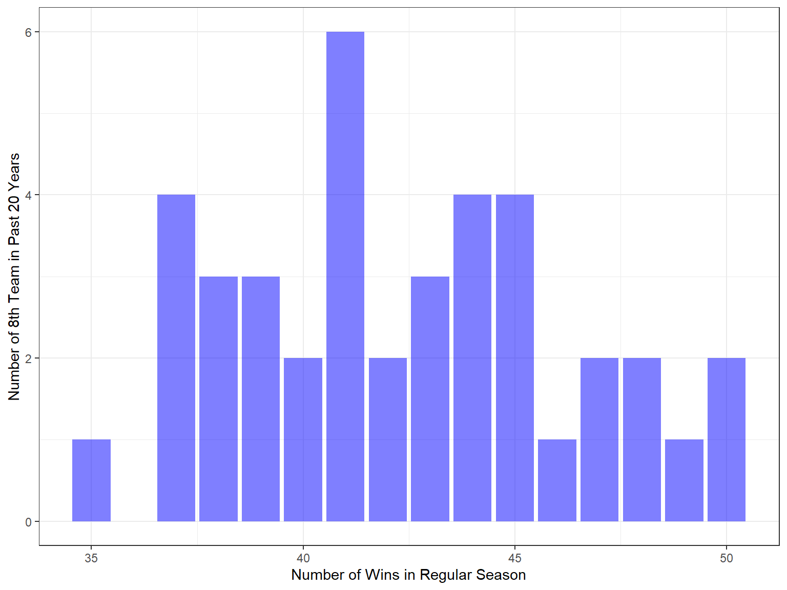
There are 40 observations of threshold in the past 20 years, which follows a normal distribution with mean 42.35 and variance 15.4641026.
Then we are going to deep dive the factors associated with the number of wins per season for a team and try to find significant contributors to increase the number of wins.
Difference in Average Scores
We wanted to look at how the scores of each play distributed in the last 10 seasons from the aspects of team which got into play-off season and team who didn’t.
non_play_off =
  box_score_viz %>%
  filter(play_off_team == "non-playoff")

box_score_viz %>%
  filter(play_off_team == "playoff") %>%
  ggplot(aes(x = pts, y = season_year)) +
  geom_density_ridges(scale = .8, alpha = .5, fill = "blue",
                      quantile_lines = T, quantile_fun = mean) +
  geom_density_ridges(data = non_play_off, aes(x = pts, y = season_year),
                      scale = .8, alpha = .5, fill = "salmon",
                      quantile_lines = T, quantile_fun = mean) +
  scale_fill_manual(name = "Team", values = cols) +
  xlim(65, 140) +
  labs(x = "Scores",
       y = "Season Year",
title = "Score Distribution Between Playoff and Regular Season Team") 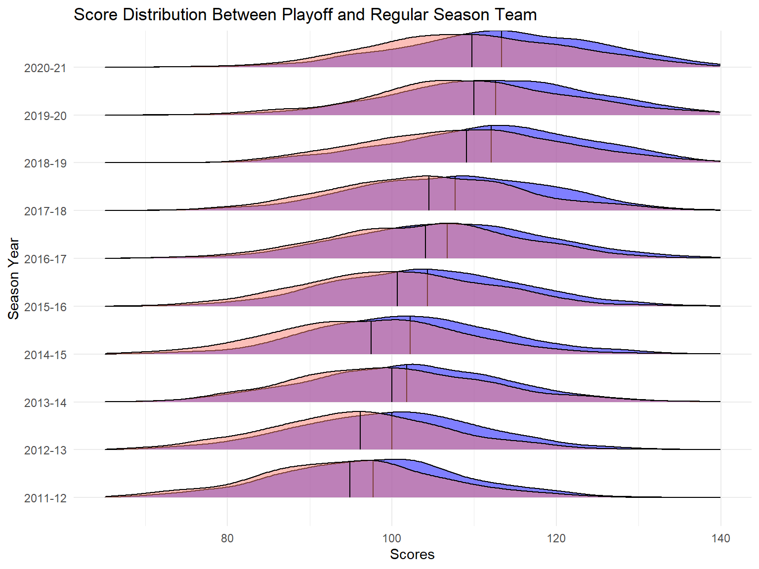
From the above ridge plot, firstly, in the last 10 regular seasons, score of each play displays an increasing trend. Secondly, team who got into the playoff season have higher average scores compared to team who did not get into playoff season.
It’s easy to understand that playoff teams outscore the non-plyoff teams because higher scores let them win more. As for the rising of average score for all NBA teams, that is due to the small ball revolution, in which teams are going to speed up, get more shooting chances and increase the percentage of three points shooting.
Three Point Parameters
Next, we use the Boxscore data and team average data to deep dive potential variables that contribute to the wining of plays.
It is clear that the percentage of three point field goal attempt in all field goal attempt were increasing in the last 10 seasons, which corresponds to the phenomenon of “Small Ball Revolution” and our analysis that score of each play was increasing in last 10 regular seasons. On the other hand, team who got into playoff season have more three point shooting attempt during a game, which means the percentage of three point shooting attempt might be a contributor to the number of game wins.
Moreover, the three pointer rate is higher among playoff teams than non-playoff teams. That is because high shooting rate corresponds to higher scores of a game. Another tendency from this plot is that the variation of three point shooting rate has reduced, which reflects the fact that teams paid more attention to three point shooting. If players were trained more on shooting, their shooting would become more stable.
Three Field Goal Attempt Percent
plot_ly(box_score_viz, x = ~ season_year, y = ~ fg3a_p, color = ~ play_off_team, type = "box") %>%
  layout(boxmode = "group",
         xaxis = list(title = 'Season Year'),
         yaxis = list(title = "Three Field Goal Attempt Percent"))
Three Point shooting Rate
plot_ly(box_score_viz, x = ~ season_year, y = ~ fg3p, color = ~ play_off_team, type = "box") %>%
  layout(boxmode = "group",
         xaxis = list(title = 'Season Year'),
         yaxis = list(title = "Three Pointer Rate"))
Offensive Play Type
Then, we want explore how offensive play type can influence the number of wins. If a playtype can apparently contribute to the number of wins of a team, we would suggest Knicks to design more offense in that type.
The average isolation per game in playoff teams are almost equal from 2013-14 seasaon to now, while the average isolations per game for non-playoff teams tended to decrease overtime. “Super star group” might account for this phenomenon, because super stars are able to conduct more isolation offense. As super stars joined the playoff team, the isolation of non-playoff teams decreased.
Pick and roll is a common offensive team work.The average pick and rolls per game tended to increase in the last 8 years for both type of teams. The number of play and roll for playoff teams was lower than that of non-playoff teams, which matched the phenomenon of isolation a lot.
Transition means the defensive team immediately launches a fast break after getting the rebound or stealing the ball without waiting for the new defensive team to be seated. It is an important way to speed up and score easily and quickly. Average transitions rose gradually because it is more efficient. And non-playoff teams seemed to conduct more transitions than playoff teams. But that didn’t mean more transitions less wins, instead it was likely that due to the team was non-playoff team, it has lower power in seated offense thus they tended to do more transitions.
Isolation
play_tp_df %>%
  group_by(season_year, play_off_team) %>%
  summarise(iso_mean = mean(poss_iso)) %>%
  mutate(text_label = str_c("Team Type: ", play_off_team,
                            "\nAverage Isolation: ", round(iso_mean, 2))) %>%
  plot_ly(x = ~ season_year, y = ~ iso_mean, type = "bar",
    color = ~ play_off_team, text = ~text_label, colors = "viridis") %>%
  layout(barmode = "group",
         xaxis = list(title = 'Season Year'),
         yaxis = list(title = "Average Isolation"))
Pick and Roll
play_tp_df %>%
  group_by(season_year, play_off_team) %>%
  summarise(pr_mean = mean(poss_pr)) %>%
  mutate(text_label = str_c("Team Type: ", play_off_team,
                            "\nAverage Pick and Roll: ", round(pr_mean, 2))) %>%
  plot_ly(x = ~ season_year, y = ~ pr_mean, type = "bar",
    color = ~ play_off_team, text = ~text_label, colors = "viridis") %>%
  layout(barmode = "group",
         xaxis = list(title = 'Season Year'),
         yaxis = list(title = "Average Pick and Roll"))
Transition
play_tp_df %>%
  group_by(season_year, play_off_team) %>%
  summarise(trans_mean = mean(poss_trans)) %>%
  mutate(text_label = str_c("Team Type: ", play_off_team,
                            "\nAverage Transition: ", round(trans_mean, 2))) %>%
  plot_ly(x = ~ season_year, y = ~ trans_mean, type = "bar",
    color = ~ play_off_team, text = ~text_label, colors = "viridis") %>%
  layout(barmode = "group",
         xaxis = list(title = 'Season Year'),
         yaxis = list(title = "Average Transition"))
Season Average Movement Parameters
Block is a key defense parameter. Higher blocks mean that your opponents have lower chance to score on you. Playoff teams played better on blocks than non-playoff teams.
Steal is also a defense parameter, which is accompanied by turnovers of opponents. There was no apparent tendency in steal over time.
Too many turnovers would let a team lose a game. The turnover plot shows that the average turnovers in playoff teams were lower than the average turnovers in non-playoff teams.
Defensive rebounds could prevent the opponent’s second attack so that reduce its scores. As we can see, palyoff teams could grab more defensive rebounds than non-playoff teams.
The number of passing per game reflect the offense fluency. Adequate number of passes could bring create good shooting opportunities, but no good shooting opportunity created after too many passes represents bad offense ability. From the passes plot, non-playoff teams had higher average passes per game than playoff teams.
Block
avg_viz_df %>%
  group_by(season_year, play_off_team) %>%
  summarise(blk_mean = mean(blk)) %>%
  mutate(text_label = str_c("Team Type: ", play_off_team,
                            "\nAverage Block: ", round(blk_mean, 2))) %>%
  plot_ly(x = ~ season_year, y = ~ blk_mean, type = "bar",
    color = ~ play_off_team, text = ~text_label, colors = "viridis") %>%
  layout(barmode = "group",
         xaxis = list(title = 'Season Year'),
         yaxis = list(title = "Average Steal"))
Steal
avg_viz_df %>%
  group_by(season_year, play_off_team) %>%
  summarise(stl_mean = mean(stl)) %>%
  mutate(text_label = str_c("Team Type: ", play_off_team,
                            "\nAverage Steal: ", round(stl_mean, 2))) %>%
  plot_ly(x = ~ season_year, y = ~ stl_mean, type = "bar",
    color = ~ play_off_team, text = ~text_label, colors = "viridis") %>%
  layout(barmode = "group",
         xaxis = list(title = 'Season Year'),
         yaxis = list(title = "Average Steal"))
Turnover
avg_viz_df %>%
  group_by(season_year, play_off_team) %>%
  summarise(tov_mean = mean(tov_avg)) %>%
  mutate(text_label = str_c("Team Type: ", play_off_team,
                            "\nAverage Turnover: ", round(tov_mean, 2))) %>%
  plot_ly(x = ~ season_year, y = ~ tov_mean, type = "bar",
    color = ~ play_off_team, text = ~text_label, colors = "viridis") %>%
  layout(barmode = "group",
         xaxis = list(title = 'Season Year'),
         yaxis = list(title = "Average Turnover"))
Defensive Rebound
avg_viz_df %>%
  group_by(season_year, play_off_team) %>%
  summarise(dreb_mean = mean(dreb)) %>%
  mutate(text_label = str_c("Team Type: ", play_off_team,
                            "\nAverage Defensive Rebound: ", round(dreb_mean, 2))) %>%
  plot_ly(x = ~ season_year, y = ~ dreb_mean, type = "bar",
    color = ~ play_off_team, text = ~text_label, colors = "viridis") %>%
  layout(barmode = "group",
         xaxis = list(title = 'Season Year'),
         yaxis = list(title = "Average Turnover"))
Passes
avg_viz_df %>%
  group_by(season_year, play_off_team) %>%
  summarise(passes_mean = mean(passes_made)) %>%
  mutate(text_label = str_c("Team Type: ", play_off_team,
                            "\nAverage Passes: ", round(passes_mean, 2))) %>%
  plot_ly(x = ~ season_year, y = ~ passes_mean, type = "bar",
    color = ~ play_off_team, text = ~text_label, colors = "viridis") %>%
  layout(barmode = "group",
         xaxis = list(title = 'Season Year'),
         yaxis = list(title = "Average Passes"))
Regression
In this part, we are going to use linear model to quantify the relationship between the number of wins and average performance parameters. Further, to know the factors influencing the result of a single game, we also use logistic regression to fit the box score data.
MLR exploration
Correlation Matrix
predict_df %>%
  select(-fg3a_total, -fg3m_total, -play_off_team, -conf_rank) %>%
  ggpairs(columns = 4:16)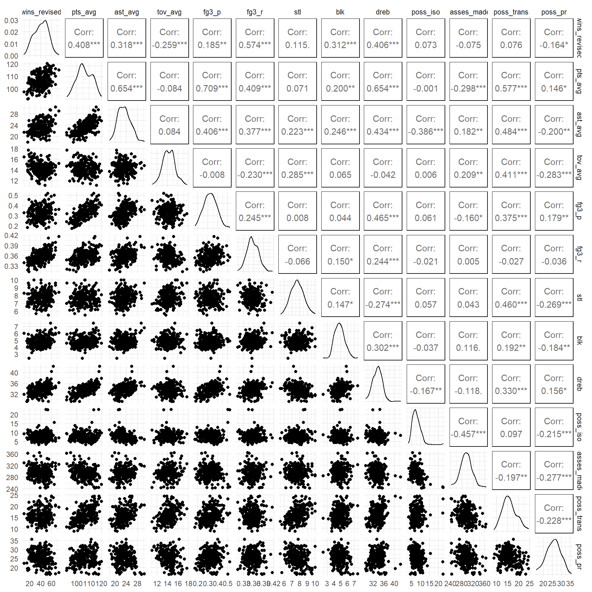
The correlation between predictors are not very high, which is important for preventing collinearity.
We used backward elimination method to select the significant dependents. Firstly, put all the potential variables into the linear model, click here to see the regression results.
model1 = lm(data = predict_df, wins_revised ~ pts_avg + tov_avg + fg3_p + fg3_r + stl + blk + dreb + poss_trans + poss_iso + poss_pr + ast_avg + passes_made)The adjusted R square for the full model is 0.5767 that is to say 57.67% of variances in the response variable can be explained by the predictors.
Then, to get a better model with higher adjusted R square, we delete the less effective predictors with higher p-value, which is passes_made. The resulting model is model2
model2 = lm(data = predict_df, wins_revised ~ pts_avg + tov_avg + fg3_p + fg3_r + stl + blk + dreb + poss_trans + poss_iso + poss_pr + ast_avg)The adjusted R square got improved to 0.5777. 57.77% of variances in the response variable can be explained by the predictors.
The result shows that assistance may not be a variable that significantly impacts the number of winings, so we decide to delete this variable from our model
model3 = lm(data = predict_df, wins_revised ~ pts_avg + tov_avg + fg3_p + fg3_r + stl + blk + dreb + poss_trans + poss_iso + poss_pr)
model3 %>% broom::tidy() %>% knitr::kable()| term | estimate | std.error | statistic | p.value |
|---|---|---|---|---|
| (Intercept) | -185.1802187 | 21.7897670 | -8.498495 | 0.0000000 |
| pts_avg | 0.3251935 | 0.1946784 | 1.670414 | 0.0962036 |
| tov_avg | -2.0555801 | 0.5646676 | -3.640337 | 0.0003366 |
| fg3_p | -22.3063836 | 11.5346505 | -1.933859 | 0.0543629 |
| fg3_r | 270.4523865 | 37.1830136 | 7.273547 | 0.0000000 |
| stl | 5.6946036 | 0.8515696 | 6.687185 | 0.0000000 |
| blk | 0.9850197 | 0.8078006 | 1.219385 | 0.2239526 |
| dreb | 3.3423210 | 0.4578976 | 7.299276 | 0.0000000 |
| poss_trans | -1.1493701 | 0.3017334 | -3.809223 | 0.0001791 |
| poss_iso | 0.6970955 | 0.2287848 | 3.046949 | 0.0025830 |
| poss_pr | -0.6435787 | 0.1555634 | -4.137083 | 0.0000494 |
The adjusted R square got decreased to 0.5768, but the difference is not significant. But consider the criteria of parsimony, we still exclude assistance from our model. In addition, block is also a variable that has a high p value. However, consider blocks is a important parameter in evaluating the defense level, it would be included in our model.
Cross Validation
With respect to the above three models, we want to see which model has the best generalizability. So in this section, cross validation is used to compare candidate model
set.seed(1000)

predict_cv_df =
  predict_df %>%
  crossv_mc(100) %>%
  mutate(train = map(train, as.tibble),
         test = map(test, as.tibble))

predict_cv_df =
  predict_cv_df %>%
  mutate(model1 = map(train, ~lm(wins_revised ~ pts_avg + ast_avg + tov_avg + fg3_p + fg3_r + stl + blk + dreb + poss_trans + passes_made + poss_iso + poss_pr, data = .x)),
         model2 = map(train, ~lm(wins_revised ~ pts_avg + ast_avg + tov_avg + fg3_p + fg3_r + stl + blk + dreb + poss_trans + poss_iso + poss_pr, data = .x)),
         model3 = map(train, ~lm(wins_revised ~ pts_avg + tov_avg + fg3_p + fg3_r + stl + blk + dreb + poss_trans + poss_iso + poss_pr, data = .x))) %>%
  mutate(rmse1 = map2_dbl(model1, test, ~rmse(model = .x, data = .y)),
         rmse2 = map2_dbl(model2, test, ~rmse(model = .x, data = .y)),
         rmse3 = map2_dbl(model3, test, ~rmse(model = .x, data = .y)))


predict_cv_df %>%
  select(starts_with("rmse")) %>%
  pivot_longer(everything(),
               names_to = "model",
               names_prefix = "rmse",
               values_to = "rmse") %>%
  ggplot(aes(x = model, y = rmse, fill = model)) +
  geom_boxplot(alpha = .6)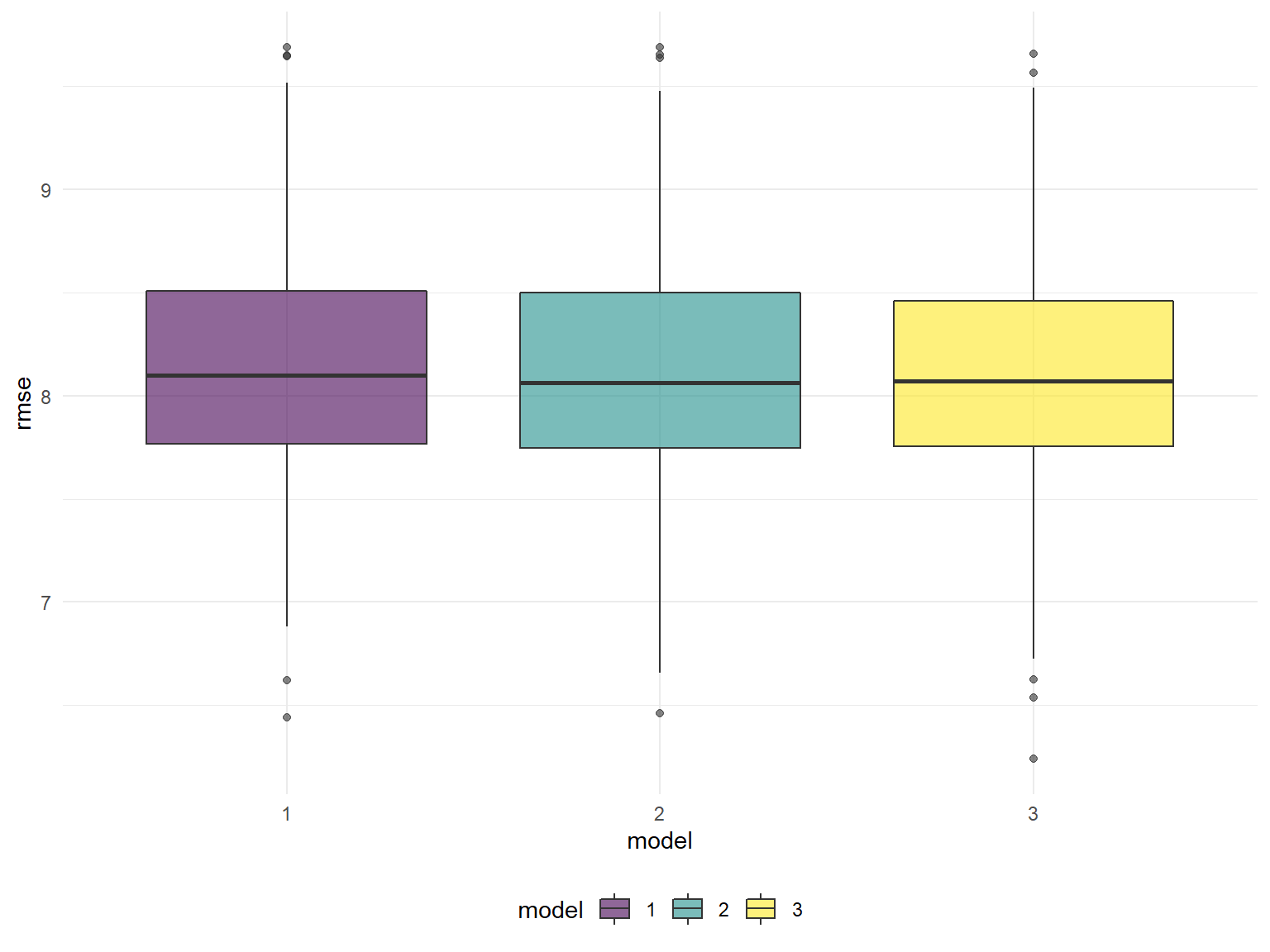
The results rmse distribution of the three model are very similar to each other, which indicates similar level of generalizability. Therefore, we still use the model3 for the final model.
Model diagnostic
We can see that Residuals vs Fitted is approximately normally distributed around 0. On the other hand, heteroscedasticity is not a problem in this model. And there is no out-lier that have big impact on the model fit.
par(mfrow=c(2,2))
plot(model2, which = 1)
plot(model2, which = 2)
plot(model2, which = 3)
plot(model2, which = 4)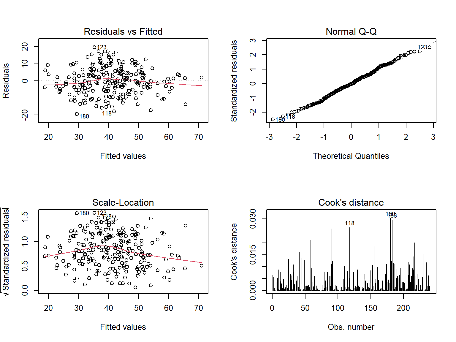
Interpretation of model coefficients
Our final model is model 3, below shows the result
\[wins\_revised = -185 + 0.33(pts\_avg) – 2.06(tov\_avg) – 22.3(fg3\_p) + 270(fg3\_r) + 5.69(stl) + 0.99(blk) \\+ 3.34(dreb) – 1.15(poss\_trans) + 0.7(poss\_iso) – 0.64(poss\_pr)\]
model3 %>% broom::tidy() %>% knitr::kable()| term | estimate | std.error | statistic | p.value |
|---|---|---|---|---|
| (Intercept) | -185.1802187 | 21.7897670 | -8.498495 | 0.0000000 |
| pts_avg | 0.3251935 | 0.1946784 | 1.670414 | 0.0962036 |
| tov_avg | -2.0555801 | 0.5646676 | -3.640337 | 0.0003366 |
| fg3_p | -22.3063836 | 11.5346505 | -1.933859 | 0.0543629 |
| fg3_r | 270.4523865 | 37.1830136 | 7.273547 | 0.0000000 |
| stl | 5.6946036 | 0.8515696 | 6.687185 | 0.0000000 |
| blk | 0.9850197 | 0.8078006 | 1.219385 | 0.2239526 |
| dreb | 3.3423210 | 0.4578976 | 7.299276 | 0.0000000 |
| poss_trans | -1.1493701 | 0.3017334 | -3.809223 | 0.0001791 |
| poss_iso | 0.6970955 | 0.2287848 | 3.046949 | 0.0025830 |
| poss_pr | -0.6435787 | 0.1555634 | -4.137083 | 0.0000494 |
All variables selected are significant in this linear regression model. Frome the estimation result, we can conclude that a small progress in the number of turnover, three pointer rate and defensive rebound can improve the number of wins in regular season.
If a team has one more turnover in each play on average, the team can have two more loss in the regular season, which hurts badly.
If a team can increase its three pointer rate by one percent, there will be 2.7 extra wins in the regular season, which helps the team a lot.
For each 1 additional average defensive rebound, there will be 3.34 extra wins! Protecting the defensive rebound well is critical.
What is beyond expectation is that the percentage of three field goal attempt is negatively associated with the number of result. The explanation behind this result could be that usually the three pointer rate is below 50%. Shooting more means that more chance would fall at the hand of opposite team. That is to say, more three point shots not necessarily means more wins.
For other variables such as steal, the occurrence of them in a game is very few, which is to say, it is difficult to make an improvement
Logistic Regression exploration
The box_score_all dataset contains 47830 games’ data from season 2012-2013 to season 2020-2021, which includes 30 variables. We are going to use some of them to build a logistics regression to see that what kind of variables will affect the game result. In addition we also use this data to do a linear regression for predicting the score.click here to see the regression results.
Correlation Matrix
First, we draw a correlation map to exam correlation of each variables, this process can help us select variables for building our logistic model.
regre_df =
  regre_df %>%
  mutate(
    min = as.numeric(min),
    fgm = as.numeric(fgm),
    fga = as.numeric(fga),
    fg_pct = as.numeric(fg_pct),
    fg3m = as.numeric(fg3m),
    fg3a = as.numeric(fg3a),
    fg3_pct = as.numeric(fg3_pct),
    ftm = as.numeric(ftm),
    fta = as.numeric(fta),
    ft_pct = as.numeric(ft_pct),
    oreb = as.numeric(oreb),
    dreb = as.numeric(dreb),
    reb = as.numeric(reb),
    ast = as.numeric(ast),
    tov = as.numeric(tov),
    stl = as.numeric(stl),
    blk = as.numeric(blk),
    blka = as.numeric(blka),
    pf = as.numeric(pf),
    pfd = as.numeric(pfd),
    pts = as.numeric(pts),
    plus_minus = as.numeric(plus_minus)
  )
corr <- cor(regre_df[-1])
corrplot(corr, method = "square", order = "FPC")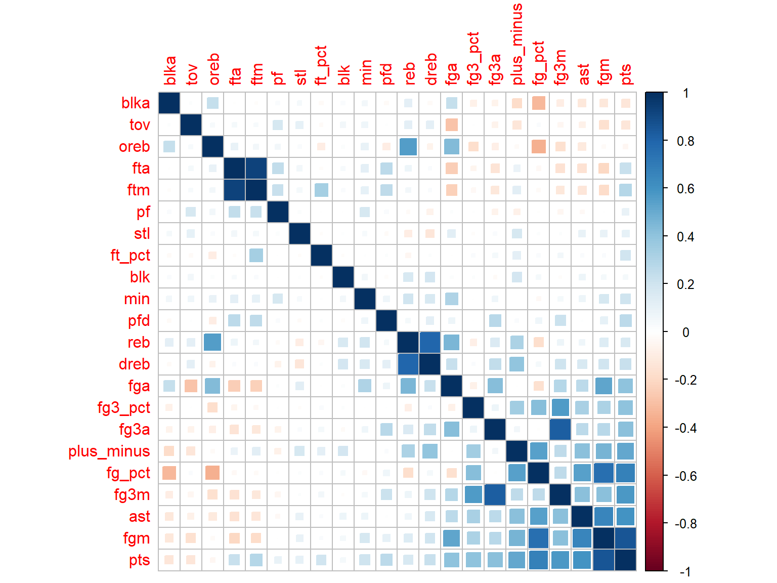
Based on this plot, we can see that there are strong correlation between some variables, like ftm and fta, dreb and reb. We will select one variable from a pair of variables that have strong correlation (which is more than 0.5). And we can select variables which have no strong correlation with others.
Modelling
Separate data as 80% training data and 20% testing data for prediction.
set.seed(22)
train.index <- sample(x = 1:nrow( regre_df), size = ceiling(0.9*nrow(regre_df)))

train = regre_df[train.index, ]
test = regre_df[-train.index, ]
Based on the correlation plot above, we choose the variables we are interested and build logistic regression model using stepwise regression.
lg_regre <- glm(wl~fg_pct+fg3_pct+ft_pct+oreb+dreb+ast+stl+blk+tov+pf,data = train, family = "binomial",control = list(maxit = 1000))
logit.step = step(lg_regre,direction = "both")
lg_regre %>% broom::tidy() %>% knitr::kable()| term | estimate | std.error | statistic | p.value |
|---|---|---|---|---|
| (Intercept) | -25.1502742 | 0.2823800 | -89.06535 | 0 |
| fg_pct | 30.3007189 | 0.3946944 | 76.77008 | 0 |
| fg3_pct | 4.3004764 | 0.1322090 | 32.52786 | 0 |
| ft_pct | 3.6269519 | 0.1339344 | 27.08006 | 0 |
| oreb | 0.1691057 | 0.0038275 | 44.18163 | 0 |
| dreb | 0.2375430 | 0.0031526 | 75.34752 | 0 |
| ast | -0.0408460 | 0.0032164 | -12.69913 | 0 |
| stl | 0.2632653 | 0.0051024 | 51.59663 | 0 |
| blk | 0.1203968 | 0.0053404 | 22.54450 | 0 |
| tov | -0.1776777 | 0.0037780 | -47.03018 | 0 |
| pf | -0.0671351 | 0.0030500 | -22.01118 | 0 |
We obtain a model with variables contain fg_pct,fg3_pct,ft_pct,oreb,dreb,ast,stl,blk,tov,pf.
Model accuracy
To evaluate the predict accuracy of this logistic regression, we now use the 20% of original data to do testing.
probabilities <- lg_regre %>% predict(test, type = "response")
# head(probabilities)
contrasts(test$wl)
predicted.classes <- ifelse(probabilities > 0.5, "1", "0")
# head(predicted.classes)
mean(predicted.classes == test$wl)## [1] 0.8053523Using the logistic model of all variables we selected, the prediction accuracy is 0.8053523.
Interpretation of model coefficients
lg_regre %>% broom::tidy() %>% knitr::kable()| term | estimate | std.error | statistic | p.value |
|---|---|---|---|---|
| (Intercept) | -25.1502742 | 0.2823800 | -89.06535 | 0 |
| fg_pct | 30.3007189 | 0.3946944 | 76.77008 | 0 |
| fg3_pct | 4.3004764 | 0.1322090 | 32.52786 | 0 |
| ft_pct | 3.6269519 | 0.1339344 | 27.08006 | 0 |
| oreb | 0.1691057 | 0.0038275 | 44.18163 | 0 |
| dreb | 0.2375430 | 0.0031526 | 75.34752 | 0 |
| ast | -0.0408460 | 0.0032164 | -12.69913 | 0 |
| stl | 0.2632653 | 0.0051024 | 51.59663 | 0 |
| blk | 0.1203968 | 0.0053404 | 22.54450 | 0 |
| tov | -0.1776777 | 0.0037780 | -47.03018 | 0 |
| pf | -0.0671351 | 0.0030500 | -22.01118 | 0 |
Our final model for predicting game result is showing below.
\[GameResult_i=-25.150274 + 30.300719 (fg\_pct)+4.300476(fg3\_pct)+3.626952(ft\_pct)+0.169106(oreb)+\\ 0.237543(dreb)-0.040846(ast)+0.263265(stl)+0.120397(blk)-0.177678(tov)-0.067135(pf)\\ i=win,lose \]
For logistic regression, we can explain variables from the perspective of odds.
All variables selected are significant in this logistic regression model.
For each additional 1 of proportion of field goals attempted, the odds of win over loss will become \(e^{30.300719}\) times.
For each additional 1 of proportion three points shooting, the odds of win over loss will become \(e^{4.300476}\) times.
For each additional 1 of proportion of free throw, the odds of win over loss will become \(e^{3.626952}\)times.
For each additional 1 of offensive rebounds per game, the odds of win over loss will become \(e^{0.169106}\) times.
For each additional 1 of defensive rebounds per games, the odds of win over loss will become \(e^{0.237543}\)times.
For each additional 1 of steals per game, the odds of win over loss will become \(e^{0.263265}\) times.
For each additional 1 of assists per game, the odds of win over loss will become \(e^{-0.040846}\) times.
For each additional 1 of blocks per game, the odds of win over loss will become \(e^{0.120397}\) times.
For each additional 1 of turnovers per game, the odds of win over loss will become \(e^{-0.177678}\)times.
For each additional 1 of personal foul per game, the odds of win over loss will become \(e^{-0.067135}\) times.
We have built both linear and logistic regression based on the NBA data. The adjusted R square for the linear regression model is 0.6916, which can explain the game score in a large extent. And the prediction of the logistic regression model is 0.8053523, which can help us to predict the result of the game correctly. There are some variables that can positively attribute to the winning of a game in both two models, like proportion of field goals attempted, proportion three points shooting and proportion of free throw, which can instruct the Knicks to pay more attention on these aspects in daily training. There is variable that can negatively attribute to the winning of a game in both two models, turnovers, which can instruct the Knicks to avoid this action in games.
Predictions on Knicks
Based on the boxscores of this season, we use model 3 to predict number of winnings for existing 30 teams. By arranging the predicted number of winnings, the Knicks is predicted to have 43.6 winnings this season and rank 8 in the season of 2021-22. According to this result, if the Knicks wants to secure a space for playoff season, it has to improve its performance and tries to win more.
top8_east =
  prediction_21_22 %>%
  head(8) %>%
  left_join(new_season_df, by = c("season_year", "team_abbreviation", "conference")) %>%
  group_by(season_year) %>%
  mutate(ranking = row_number())

top8_east %>%
  select(season_year, team_abbreviation, conference, ranking) %>%
knitr::kable("simple")| season_year | team_abbreviation | conference | ranking |
|---|---|---|---|
| 2021-22 | MIL | east | 1 |
| 2021-22 | CHA | east | 2 |
| 2021-22 | PHI | east | 3 |
| 2021-22 | BKN | east | 4 |
| 2021-22 | CHI | east | 5 |
| 2021-22 | BOS | east | 6 |
| 2021-22 | TOR | east | 7 |
| 2021-22 | ATL | east | 8 |
Gaps in Performance
Let’s see what Knicks can do to improve its performance and rush into playoff season.
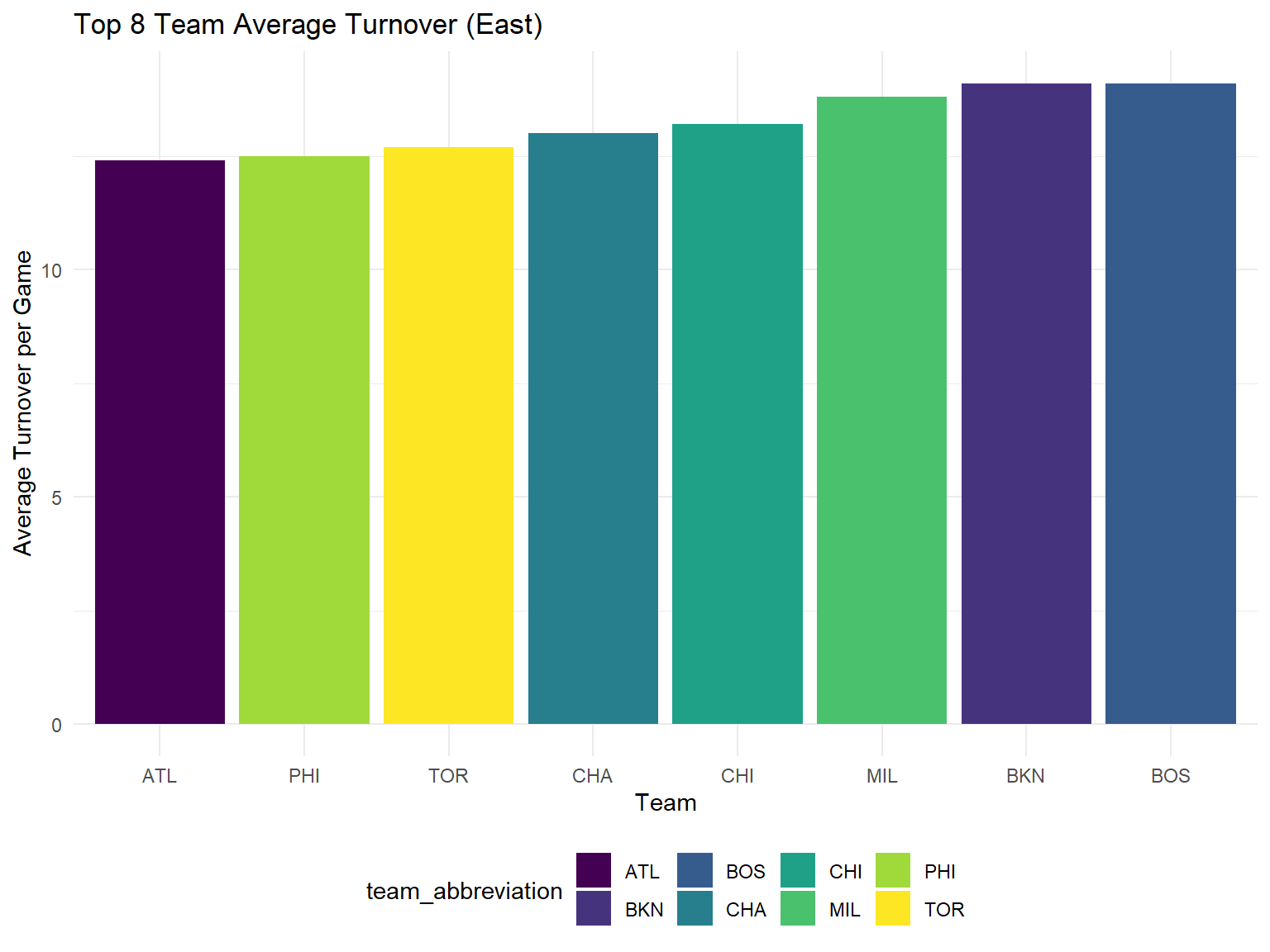
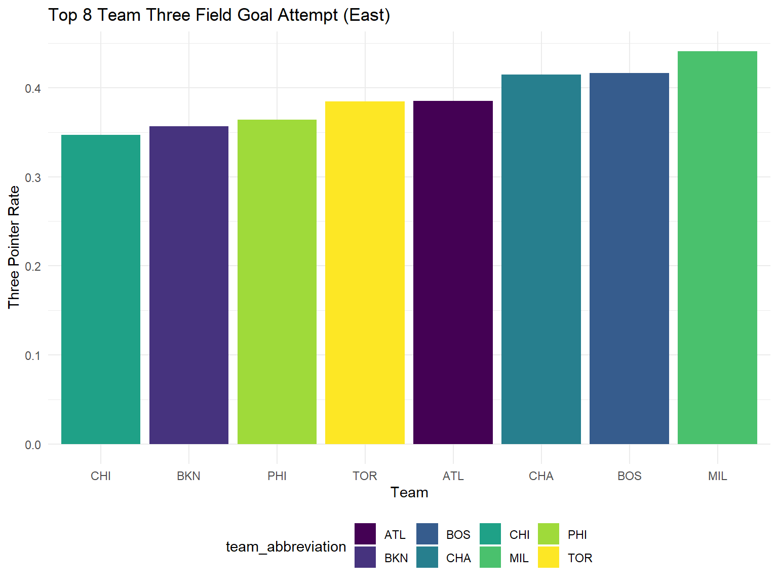
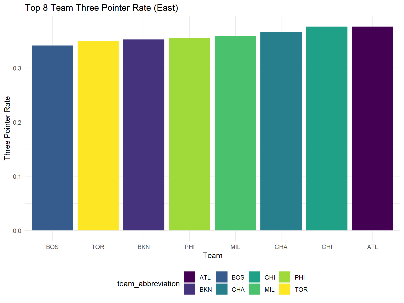
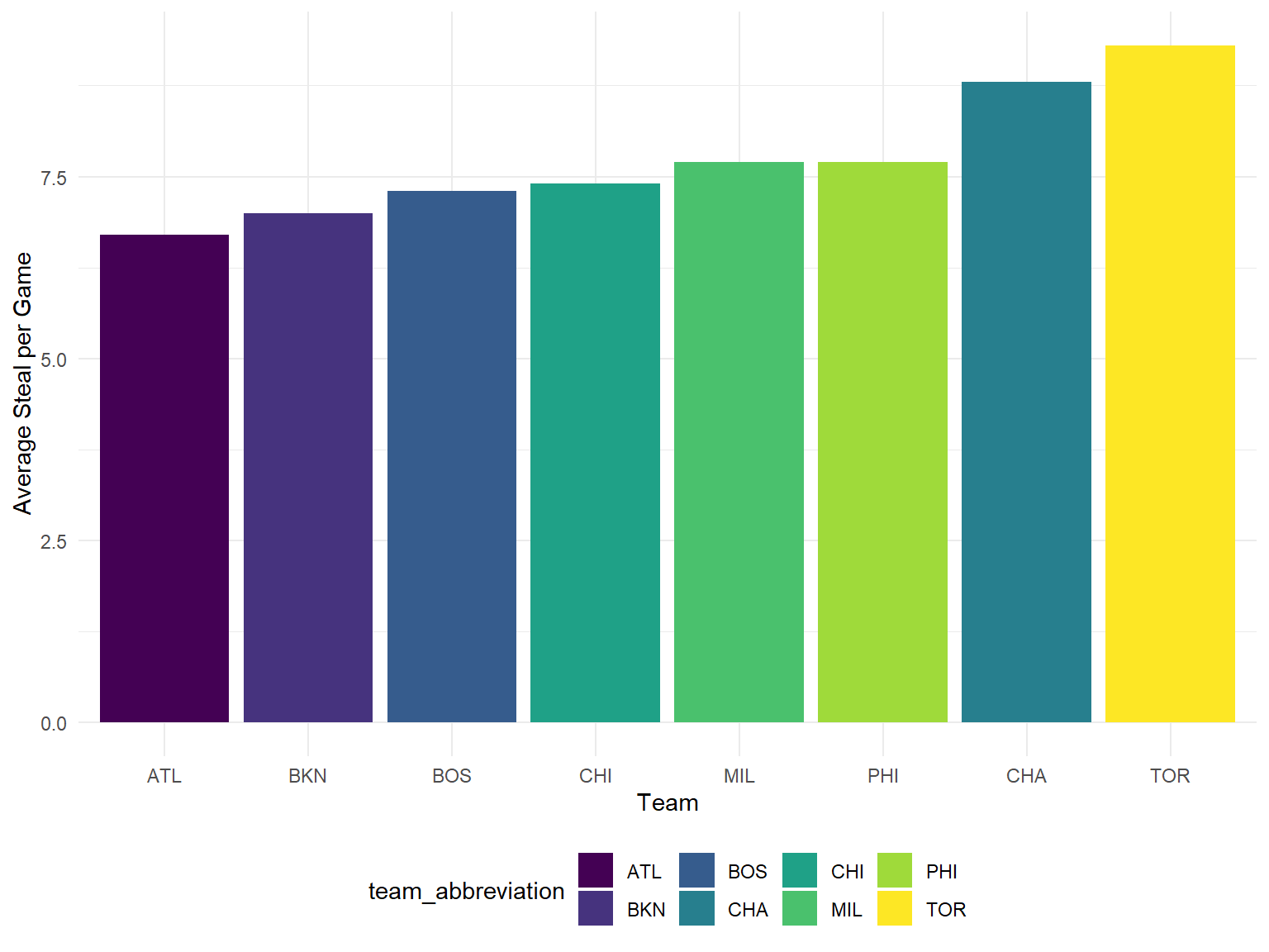
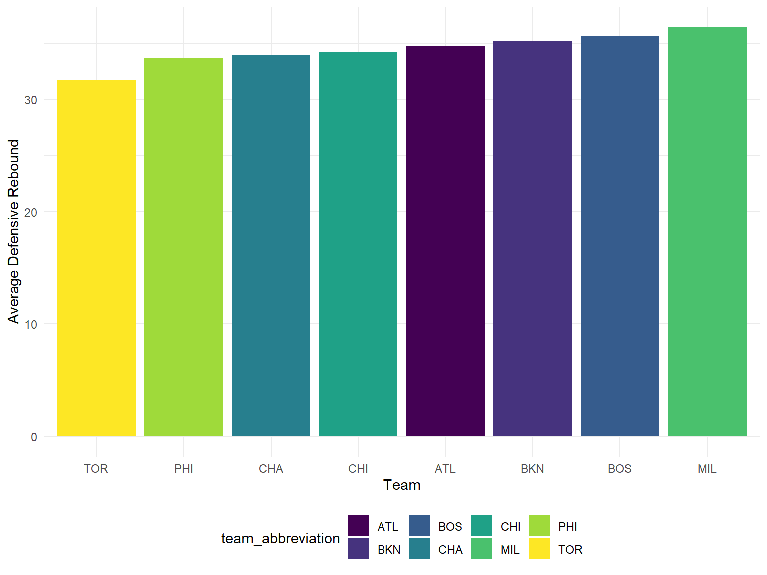
From the plots below, we can conclude that Knicks has to improve its performance in the aspects of turnover and three points. As the model shows, the number of turnover is negatively associated with the number of winning. However, Knicks currently has the second highest number of turnover per game. In addition, its high percentage of three field goal attempt and low three pointer rate among the top 8 of east conference prevent it from getting a good prediction result.
Turnover
top8_east %>%
  ggplot(aes(x = reorder(team_abbreviation, tov_avg), y = tov_avg, fill = team_abbreviation)) +
  geom_bar(stat="identity") +
  labs(
    x = "Team",
    y = "Average Turnover per Game",
    title = "Top 8 Team Average Turnover (East)"
  )
3 Field Goal Attempt Percentage
top8_east %>%
  ggplot(aes(x = reorder(team_abbreviation, fg3_p), y = fg3_p, fill = team_abbreviation)) +
  geom_bar(stat="identity") +
  labs(
    x = "Team",
    y = "Three Pointer Rate",
    title = "Top 8 Team Three Field Goal Attempt (East)"
  )
3 Pointer Rate
top8_east %>%
  ggplot(aes(x = reorder(team_abbreviation, fg3_r), y = fg3_r, fill = team_abbreviation)) +
  geom_bar(stat="identity") +
  labs(
    x = "Team",
    y = "Three Pointer Rate",
    title = "Top 8 Team Three Pointer Rate (East)"
  )
Steal
top8_east %>%
  ggplot(aes(x = reorder(team_abbreviation, stl), y = stl, fill = team_abbreviation)) +
  geom_bar(stat="identity") +
  labs(
    x = "Team",
    y = "Average Steal per Game"
  )
Defensive Rebound
top8_east %>%
  ggplot(aes(x = reorder(team_abbreviation, dreb), y = dreb, fill = team_abbreviation)) +
  geom_bar(stat="identity") +
  labs(
    x = "Team",
    y = "Average Defensive Rebound"
  )
Isolation
top8_east %>%
  ggplot(aes(x = reorder(team_abbreviation, poss_iso), y = poss_iso, fill = team_abbreviation)) +
  geom_bar(stat="identity") +
  labs(x = "Team",
       y = "Average Isolation")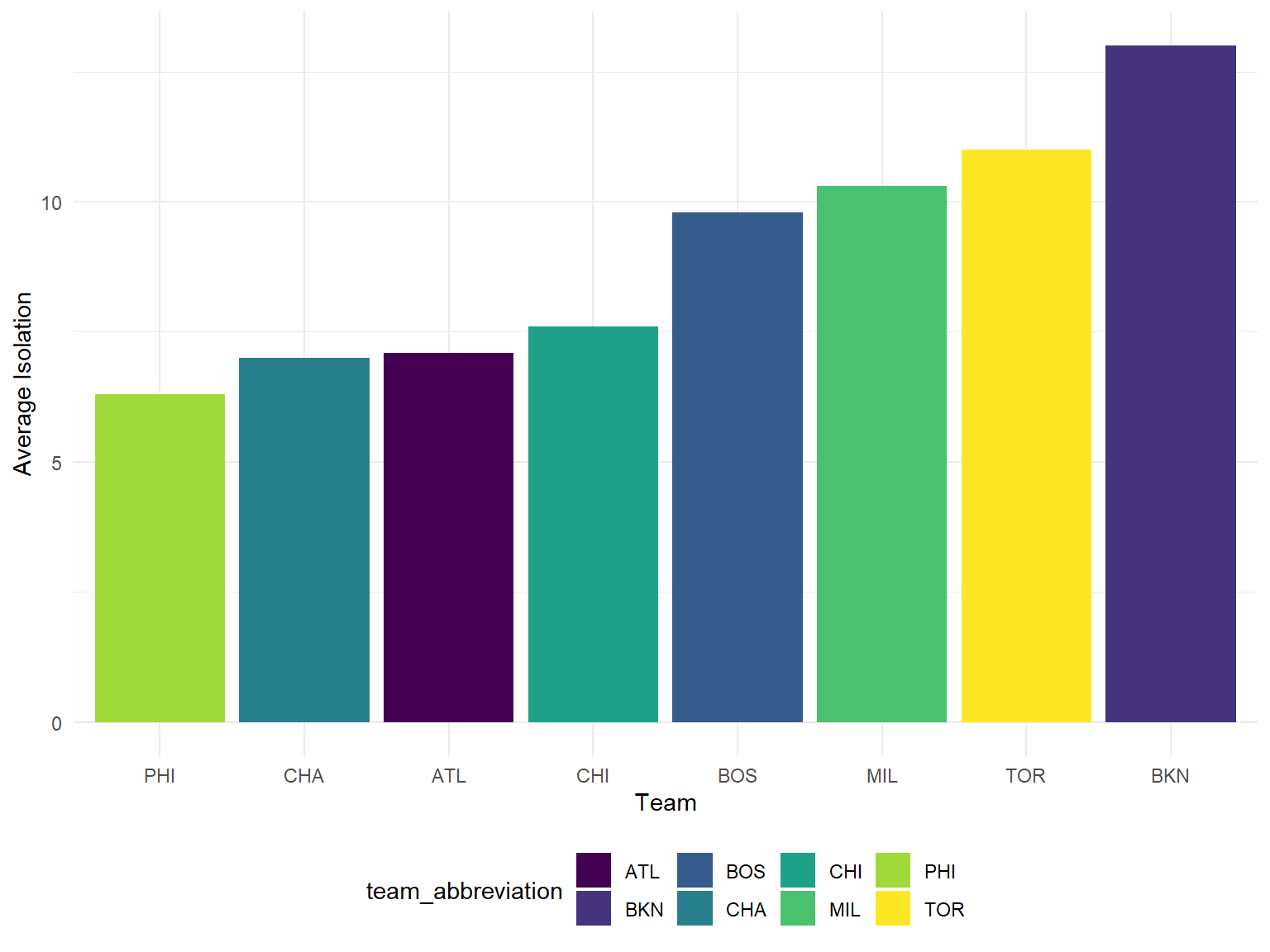
Pick and Roll
top8_east %>%
  ggplot(aes(x = reorder(team_abbreviation, poss_pr), y = poss_pr, fill = team_abbreviation)) +
  geom_bar(stat="identity") +
  labs(x = "Team",
       y = "Average Pick and Roll")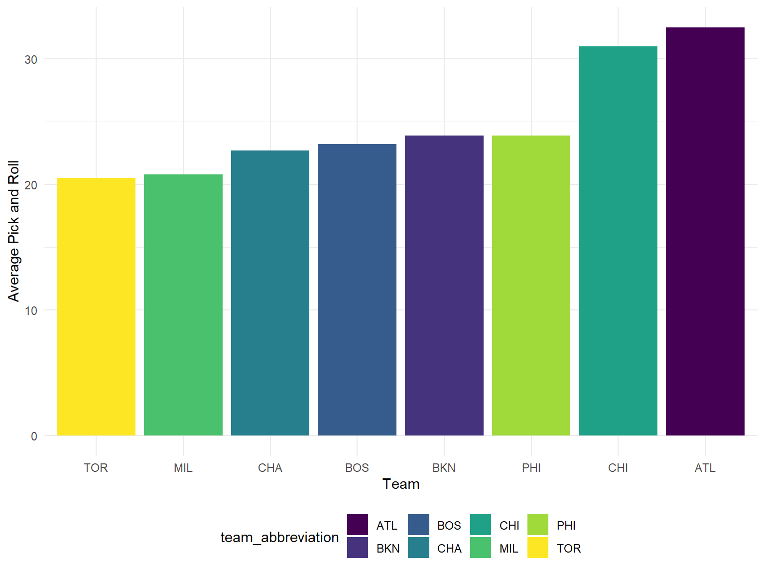
Zoom in with Three Pointer - Knicks
As three pointer is such a crutial parameter for NBA team to get into playoff season. We decide to look at Knicks’ three pointer shooting data to offer more specific suggestions. In this section, we will compare the overall performance of Knicks to league average, and then, draw the plots for some three pointer team leaders.
In this part, we referred ballr package and Owen’s blog to make the hex plots
library(prismatic)
library(extrafont)
library(cowplot)

p = plot_court(court_themes$light) +
  geom_polygon(
    data = df,
    aes(
      x = adj_x,
      y = adj_y,
      group = hexbin_id,
      fill = league_avg_diff,
      color = after_scale(clr_darken(fill, .333))),
    size = .25) +
  scale_x_continuous(limits = c(-27.5, 27.5)) +
  scale_y_continuous(limits = c(0, 45)) +
  scale_fill_distiller(direction = -1,
                       palette = "PuOr",
                       limits = c(-.15, .15),
                       breaks = seq(-.15, .15, .03),
                       labels = c("-15%", "-12%", "-9%", "-6%", "-3%", "0%", "+3%", "+6%", "+9%", "+12%", "+15%"),
                       "3FG Percentage Points vs. League Average") +
  guides(fill = guide_legend(
    label.position = 'bottom',
    title.position = 'top',
    keywidth = .45,
    keyheight = .15,
    default.unit = "inch",
    title.hjust = .5,
    title.vjust = 0,
    label.vjust = 3,
    nrow = 1))  +
  theme(legend.spacing.x = unit(0, 'cm'),
        legend.title = element_text(size = 9),
        legend.text = element_text(size = 8),
        legend.margin = margin(-10,0,-1,0),
        legend.position = 'bottom',
        legend.box.margin = margin(-30,0,15,0),
        plot.title = element_text(hjust = 0.5, vjust = -1, size = 15),
        plot.subtitle = element_text(hjust = 0.5, size = 8, vjust = -.5),
        plot.caption = element_text(face = "italic", size = 8),
        plot.margin = margin(0, -5, 0, -5, "cm")) +
  labs(title = "New York Knicks - Three Point",
       subtitle = "2021-22 Regular Season")

ggdraw(p) +
  theme(plot.background = element_rect(fill="floralwhite", color = NA))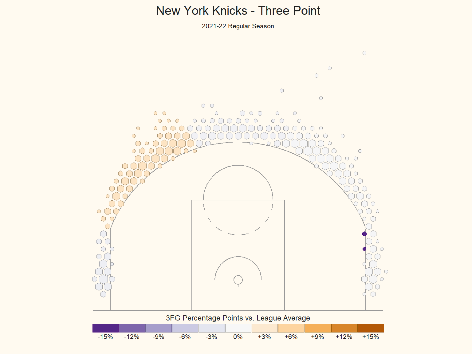
According to this hex plot, in the 2021-2022 regular season, The Knicks has a better performance in three-point field goal at both of the wing area compared to league average. And it has a equal performance with the league average at the head of the key area. However, the Knicks performs worse at the both corner area compared to the league average. To be more specific, the three pointer percentage at right wing is 6% higher than the league average. At left wing, the three pointer percentage is 3% higher than the league average. On the other hand, the team’s three pointer percentage is 6% and 3% lower than the league average in the right and left corners respectively. Therefore, the Knicks should deploy more three field goal tactics at left and right wing areas. And the shooting ability at corner area should be further strengthened through training.
Zoom in with Three Pointer - Knicks Team Leaders
As to further understand what tactic the Knicks can deploy, we decide to look at the shooting log of three pointer team leaders in Knicks, including Alec Burks, Kemba Walker and Derrick Rose, who have the highest three pointer rate in Knicks.
Alec’s Shooting
alec_p =
  plot_court(court_themes$light) +
  geom_polygon(
    data = alec_df,
    aes(
      x = hex_data.adj_x,
      y = hex_data.adj_y,
      group = hex_data.hexbin_id,
      fill = hex_data.league_avg_diff,
      color = after_scale(clr_darken(fill, .333))),
    size = .25) +
  scale_x_continuous(limits = c(-27.5, 27.5)) +
  scale_y_continuous(limits = c(0, 45)) +
  scale_fill_distiller(direction = -1,
                       palette = "PuOr",
                       limits = c(-.15, .15),
                       breaks = seq(-.15, .15, .03),
                       labels = c("-15%", "-12%", "-9%", "-6%", "-3%", "0%", "+3%", "+6%", "+9%", "+12%", "+15%"),
                       "3FG Percentage Points vs. League Average") +
  guides(fill = guide_legend(
    label.position = 'bottom',
    title.position = 'top',
    keywidth = .45,
    keyheight = .15,
    default.unit = "inch",
    title.hjust = .5,
    title.vjust = 0,
    label.vjust = 3,
    nrow = 1))  +
  theme(legend.spacing.x = unit(0, 'cm'),
        legend.title = element_text(size = 9),
        legend.text = element_text(size = 8),
        legend.margin = margin(-10,0,-1,0),
        legend.position = 'bottom',
        legend.box.margin = margin(-30,0,15,0),
        plot.title = element_text(hjust = 0.5, vjust = -1, size = 15),
        plot.subtitle = element_text(hjust = 0.5, size = 8, vjust = -.5),
        plot.caption = element_text(face = "italic", size = 8),
        plot.margin = margin(0, -5, 0, -5, "cm")) +
  labs(title = "Alec Burks - Three Point",
       subtitle = "2021-22 Regular Season")

ggdraw(alec_p) +
  theme(plot.background = element_rect(fill="floralwhite", color = NA))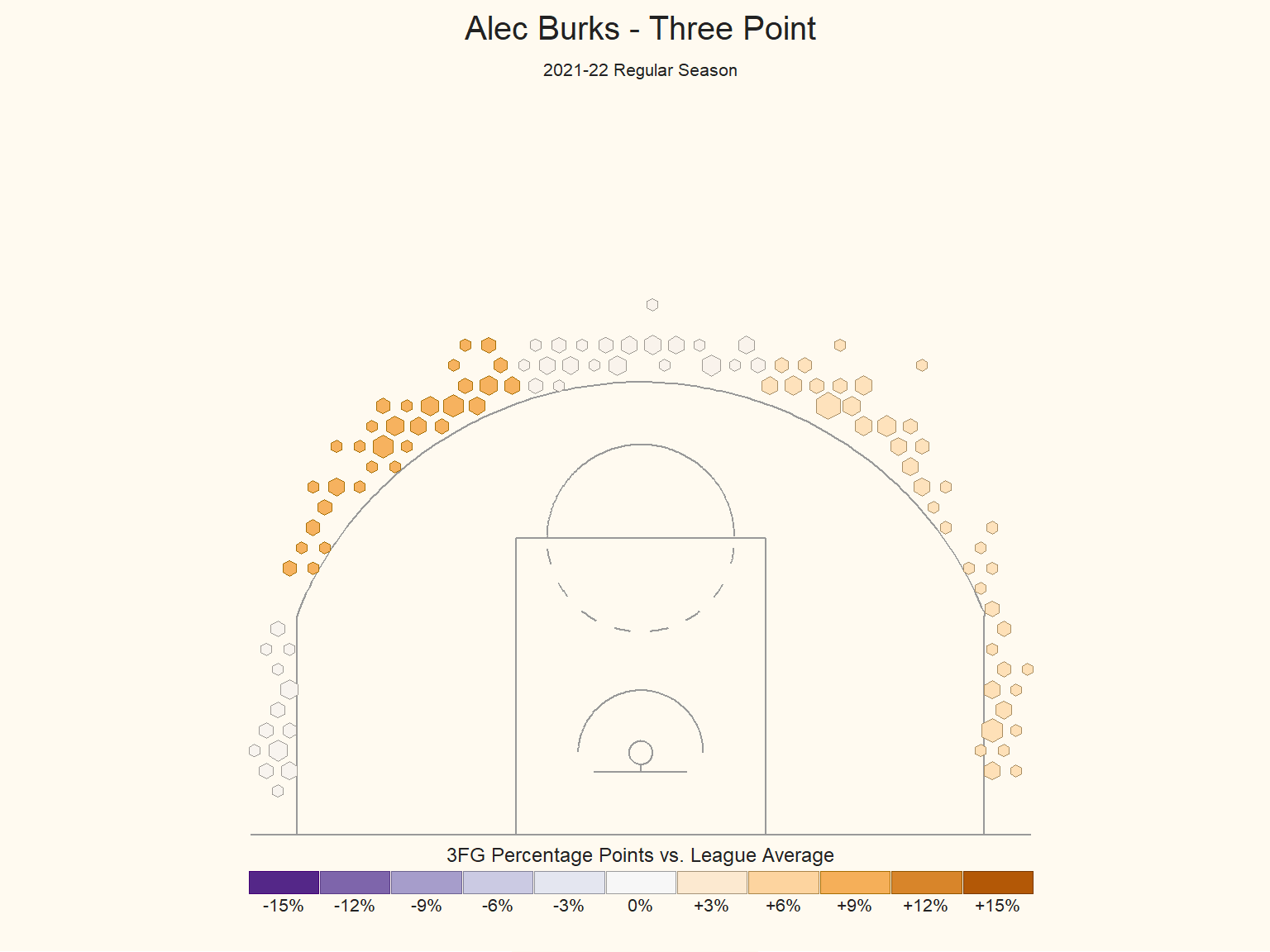
Walker’s Shooting
walker_p =
  plot_court(court_themes$light) +
  geom_polygon(
    data = walker_df,
    aes(
      x = hex_data.adj_x,
      y = hex_data.adj_y,
      group = hex_data.hexbin_id,
      fill = hex_data.league_avg_diff,
      color = after_scale(clr_darken(fill, .333))),
    size = .25) +
  scale_x_continuous(limits = c(-27.5, 27.5)) +
  scale_y_continuous(limits = c(0, 45)) +
  scale_fill_distiller(direction = -1,
                       palette = "PuOr",
                       limits = c(-.15, .15),
                       breaks = seq(-.15, .15, .03),
                       labels = c("-15%", "-12%", "-9%", "-6%", "-3%", "0%", "+3%", "+6%", "+9%", "+12%", "+15%"),
                       "3FG Percentage Points vs. League Average") +
  guides(fill = guide_legend(
    label.position = 'bottom',
    title.position = 'top',
    keywidth = .45,
    keyheight = .15,
    default.unit = "inch",
    title.hjust = .5,
    title.vjust = 0,
    label.vjust = 3,
    nrow = 1))  +
  theme(legend.spacing.x = unit(0, 'cm'),
        legend.title = element_text(size = 9),
        legend.text = element_text(size = 8),
        legend.margin = margin(-10,0,-1,0),
        legend.position = 'bottom',
        legend.box.margin = margin(-30,0,15,0),
        plot.title = element_text(hjust = 0.5, vjust = -1, size = 15),
        plot.subtitle = element_text(hjust = 0.5, size = 8, vjust = -.5),
        plot.caption = element_text(face = "italic", size = 8),
        plot.margin = margin(0, -5, 0, -5, "cm")) +
  labs(title = "Kemba Walker - Three Point",
       subtitle = "2021-22 Regular Season")

ggdraw(walker_p) +
  theme(plot.background = element_rect(fill="floralwhite", color = NA))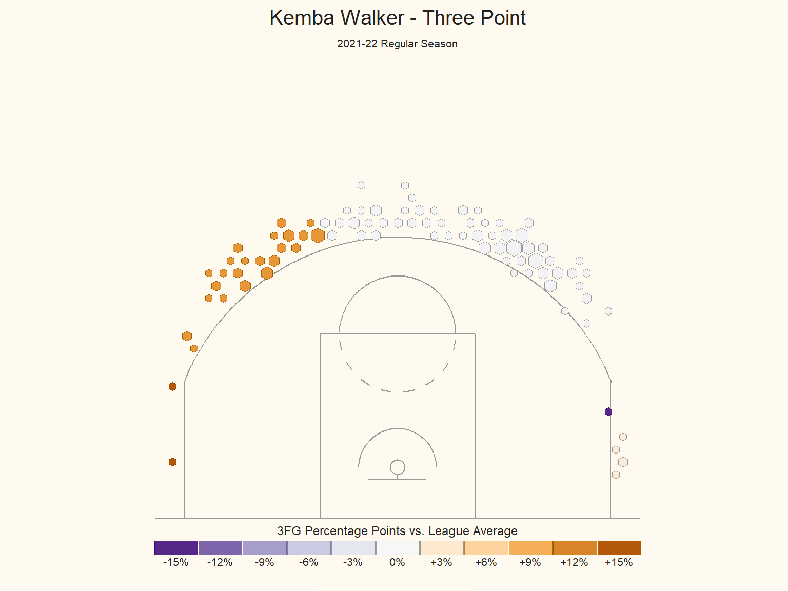
Rose’s Shooting
rose_p =
  plot_court(court_themes$light) +
  geom_polygon(
    data = rose_df,
    aes(
      x = hex_data.adj_x,
      y = hex_data.adj_y,
      group = hex_data.hexbin_id,
      fill = hex_data.league_avg_diff,
      color = after_scale(clr_darken(fill, .333))),
    size = .25) +
  scale_x_continuous(limits = c(-27.5, 27.5)) +
  scale_y_continuous(limits = c(0, 45)) +
  scale_fill_distiller(direction = -1,
                       palette = "PuOr",
                       limits = c(-.15, .15),
                       breaks = seq(-.15, .15, .03),
                       labels = c("-15%", "-12%", "-9%", "-6%", "-3%", "0%", "+3%", "+6%", "+9%", "+12%", "+15%"),
                       "3FG Percentage Points vs. League Average") +
  guides(fill = guide_legend(
    label.position = 'bottom',
    title.position = 'top',
    keywidth = .45,
    keyheight = .15,
    default.unit = "inch",
    title.hjust = .5,
    title.vjust = 0,
    label.vjust = 3,
    nrow = 1))  +
  theme(legend.spacing.x = unit(0, 'cm'),
        legend.title = element_text(size = 9),
        legend.text = element_text(size = 8),
        legend.margin = margin(-10,0,-1,0),
        legend.position = 'bottom',
        legend.box.margin = margin(-30,0,15,0),
        plot.title = element_text(hjust = 0.5, vjust = -1, size = 15),
        plot.subtitle = element_text(hjust = 0.5, size = 8, vjust = -.5),
        plot.caption = element_text(face = "italic", size = 8),
        plot.margin = margin(0, -5, 0, -5, "cm")) +
  labs(title = "Derrick Rose - Three Point",
       subtitle = "2021-22 Regular Season")

ggdraw(rose_p) +
  theme(plot.background = element_rect(fill="floralwhite", color = NA))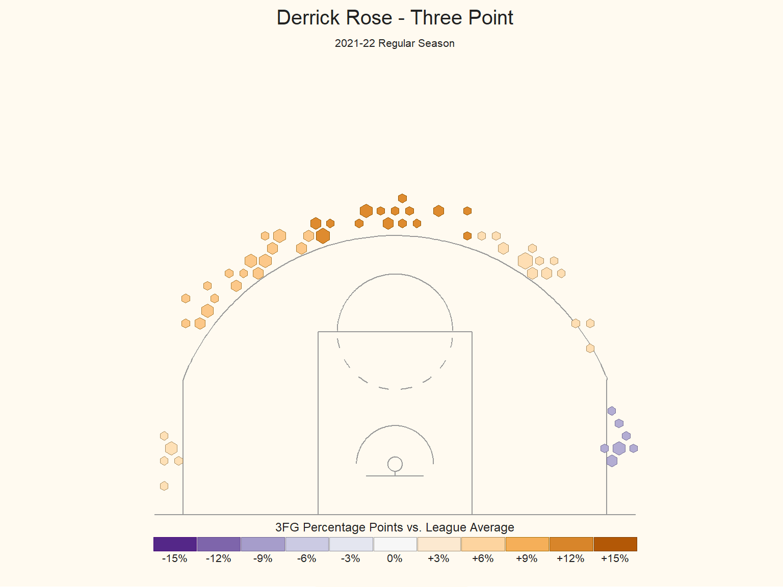
The performance of Knicks team leaders in three pointer is in accordance with the performance of the whole team. In the 2021-22 season, none of the team leaders performs better than the league average in both of the corner area.However, it is more likely for them to make three point at both wings. Therefore, we think the coach should deploy more tactics for the team leaders at wing area. And the players should make less shot attempt in a play at the corner but get more training in shooting at this area.
Shiny App
With all the data analysis and model exploration, we identified features that contribute to the number of winning in a season, game results and play scores. We think it’s necessary for the fans to see how these feature changes in different seasons for different NBA teams, moreover, make comparisons between teams. Therefore, we created an interactive dashboard in Shiny app to achieve this purpose.
In this Shiny App, users can select different feature and team(s) to visualize the team(s) performance in this feature, make comparisons and get ranking predictions for the team(s) in the season of 2021-22.
Conclusion and Discussion
Firstly, in order to enter playoff, Knicks is supposed to win about 43 games in a regular season.
Then, variables positively influencing the number of winnings a lot are mainly three points shooting rate and the average number of defense rebounds. variable negatively influencing the number o winnings a lot is the average number of turnovers.
What’s more, New York Knicks ranked second among top eight teams in the number of turnovers per game and fifth among top eight teams in the three point shooting rate. Both of the two stats are the shortage of New York Knicks. Specifically, the top three points shooting rate is slightly lower than the league average, and the corner three shooting rate is highly lower than the league average. Leading players like Alec Burks, Kemba Walker, and Derick Rose account for the low three point shooting rate.
Finally, to get more wins, we highly suggest Knicks taking advantage of the hot area, deploying more tactics in for wing three shooting. And in the training, players should practice more on corner threes. Besides, more team training is needed to avoid turnovers.